|
"Interpolation is a black art, and interpolation methods should never be trusted. Careful researchers always interpolate several times using different methods, and choose the result they dislike least." - Roger Bivand
My recently completed Master's project in Computer Science at RPI Hartford developed a computational method for the practical implementation of an interpolation
algorithm developed by Dr. Wm. Randolph Franklin at RPI Troy. The algorithm is used to interpolate terrain data from contour lines for the production of DEMs. As readers of this site are aware, sometimes this is the only method available for obtaining high resolution DEMS outside of the USA, Canada, some parts of Western Europe and those areas covered by ASTER.
Although Dr. Franklin offers one of the most accurate interpolation algorithms yet developed for this purpose, the system of linear equations required to solve it for typical cartographic data sets can be quite
large, i.e. millions of equations with millions of unknowns. The data structures to hold coefficient matrices for practical cartographic systems can easily exceed 1000 GB in size.
Fortunately, these matrices are always sparse, meaning they are populated with mostly zeros. It is possible to store such data in structures called sparse
matrices whereby only the array indices and values of the non zero elements are stored. This reduces the memory requirement considerably. However, the result is still a very large
problem, both from a storage and from a computational perspective.
My project implemented the algorithm for large input elevation grids of up to 1201 by 1201 elevation postings. A variety of techniques were originally envisioned,
including MATLAB sparse solvers, sparse libraries such as SparseLib++, and multigrid iterative methods. Ultimately, I decided upon a two level iterative approach using the Paige-Saunders conjugate gradient solver with a Laplacian central difference approximation solver used to prepare the initial estimate.
In the process, I discovered the power of iterative solvers, as well as their problems, the details of which are described in the project report.
I also compared the Franklin approximation algorithm to one commercial and one research-grade contour to DEM interpolator with additional interesting results.
A brief introduction extracted from my project proposal is shown below. My final report is available by clicking on the link below.
1.0 Statement of the problem to be solved.
The goals of the three credit Master’s Project were:
To extend the work described in the Franklin paper entitled ‘Applications of Analytical Cartography’ [1]
Demonstrate the feasibility of the algorithm described in that paper when applied to larger datasets approaching commonly used DEM formats (for example input files of 1201 by
1201 elevation grid nodes.)
Compare the results of the algorithm with commercial implementations of contour-to-grid interpolations, for example: RV2, GRASS, PCI, etc.
2.0 Significance of the problem, project justification.
Interpolating information from known data to unknown data points is one of the classical problems of computational cartography and is used widely in many diverse
GIS (Geographical Information Systems) applications. One example is the derivation of DEMs (Digital Elevation Models) from topographical contour maps for areas where DEMs are not available. In order
to do this, DEMs are sometimes reverse-engineered from contour map data. In this multi step process, contour maps are scanned into digital format if they are not already archived that way. Then the
contour line elevation data is separated from the other information on the map. The contour line data is then conditioned (to the degree possible) to correct bleeding, breaks, spurs bridges and other
anomalies.
The contours must then be tagged with their elevation data in a machine-readable format. This is typically done by vectorizing the contour lines and tagging the
vectors with their elevations either automatically, or more commonly using a semi-automated labor-intensive process. The tagged vector data is then rasterized and transferred to grid using an
interpolation algorithm. Finally, the gridded elevation values are written to some type of GIS format that can be used by other applications. The interpolative step in the process is the focus of
this proposal.
One algorithm for the interpolation (or rather the approximation) of known elevations to a regular grid is described by Dr. Franklin in the previously cited
paper. The algorithm is based on a novel application of the Laplacian PDE (partial differential equation) whereby a system of over determined linear equations is formulated and solved by performing a
linear least squares fit to the known data and unknown grid nodes.
The algorithm has several advantages as compared to previous algorithms:
It does not require continuous contours; i.e. it can deal with breaks, such as those that commonly occur when contours are too closely spaced.
It can use isolated point elevations if known, such as mountain tops.
If continuous contours with many points are available, it can use all the points (without needing to sub sample them).
Information flows across the contours, causing the slope to be continuous and the contours not to be visible in the generated surface.
If local maxima, such as mountain tops, are not given, it interpolates a reasonable bulge. It does not just put a plateau at the highest
contour.
Unlike some other methods, it works even near kidney-shaped contours, where the closest contour in all four cardinal directions might be the same
contour.
It has the advantage of producing a surface virtually free of the negative artifacts associated with other interpolation algorithms, for example terracing and
ringing.
It also offers the advantage of allowing the surface smoothness and fit to be adjusted by selective weighting of the equations corresponding to the known
elevations, thereby allowing grid adjustments to be made on a node-by-node basis if desired.
Although the algorithm offers advantages, it presents computational challenges as well. If the elevation grid is N by N postings large, the solution is formulated in terms of a
N2 by N2 coefficient matrix. Since the number of flops for row reduction for an N by N matrix is approximately 2N3/3, the time complexity for an N2 by
N2 matrix by the direct solution is 2(N2)3 /3 ~ N6. Because the proposed system is overdetermined, additional matrix multiplications are required to solve the system by least squares, increasing the computational time and storage requirements even more.
The algorithm has previously been implemented by Franklin using MATLAB on data sets of the order of 257 by 257 nodes using sparse matrix techniques. Although this was sufficient to
demonstrate the feasibility of the algorithm, real data sets are larger. It is proposed to attempt to demonstrate the algorithm on realistic data sets, as large as 1201 by 1201 grid postings. The
task is made difficult by the rapid increase in problem size as a function of the number of input elevation grid nodes. It is further proposed to compare the quality of the output grids produced by the algorithm with other
algorithms commercially implemented. In doing so, we hope to offer Dr. Franklin’s useful algorithm to the cartographic community.
A more in-depth explanation is contained in my Final Report. The latest revision of my C++ implementation of the algorithm is called BLACKART
For additional information on converting contour lines to terrains see my article entitled DEMs from Topos. and the Pierre Soille article entitled From Scanned Topographic Maps to Digital Elevation Models.
Dr. Franklin's website contains a wealth of information regarding the field of computational cartography
See the article: Mountain Gorilla Protection: A Geomatics Approach for an example of contour line interpolation and other advanced terrain modeling techniques used in a scientific application.
| 
![[Typical Input Data File. Click to enlarge]](http://www.terrainmap.com/data.jpg)
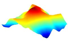
![[Crater.dat Interpolation. Click to enlarge]](http://www.terrainmap.com/crater.jpg)
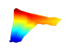
![[bountiful.dat Interpolation. Click to enlarge]](http://www.terrainmap.com/bountif_blackart.jpg)