My previous article entitled "DEMs from Topos" described a method for creating DEMs from topographic maps. This technique is useful when no other practical source of DEMs exists, or when the available DEMs are of too low a resolution.

The technique described in the article had two main problems. The first was that it used the application R2V to extract the DEM from the contour map. This program is fairly expensive, being advertised t $1495 the last time I checked the web site.

The second problem is that the R2V interpolation algorithm, as discussed in my Master's Project Final Report, appeared less than optimal. This can be seen from the example DEM that I produced when writing that article. It suffers from severe terracing, a common problem with naive interpolation algorithms.

As described on another article on this web site, I have written an implementation of a much better contour line interpolation algorithm, the Franklin over determined Laplacian approximation. The first release of this code, first as a console application and later as a GUI application was research grade software meant to demonstrate the advantages of the algorithm. However, it was not very useful because it provided no way to prepare the input file required for the interpolation (among other deficiencies.)

The release of the software that accompanied the writing of this article has solved this problem to some degree. It is capable of reading the Arc View .shp file produced by the low cost WinTopo Pro raster to vector conversion application. While not free either, the price of this application is more reachable to many people at about $200. With this investment in WinTopo, and the free BLACKART application you can produce DEMs from topo maps arguably as easily as with R2V. In addition, the quality of the interpolations produced will be very good indeed, as the Franklin algorithm is perhaps the best currently available for this purpose. I will attempt in this article to demonstrate how this can be done.

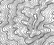
The first step is to acquire a raster topo image as input to WinTopo. These are extracted from topographic maps. Since I described a couple of ways to do this in the earlier article, I will not repeat them here. I will use the "topo.tif" test image included with the R2V demonstration distribution. This image contains fairly clean contour lines and does not require a lot of preparatory work which saves me time in putting together this article. Extracting and cleaning the input raster image is a large part of the effort involved in making DEMs from topos.

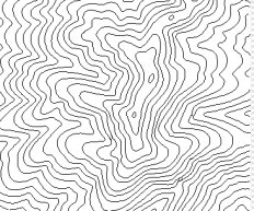
A relatively small section of this image is shown to the right. In WinTopo, you prepare the image by first thinning the contour lines using one of the algorithms provided under the "Image" menu selection. After thinning, use the magnifying icon to examine the image for broken, bleeding, touching, or crossed contour lines. Use the eraser tool and drawing tool to correct all of these and also any unwanted spurs, stray pixels or other unwanted artifacts. It is important to spend the time to correct all of these flaws carefully as this is the only way to produce a high quality product from your efforts. WinTopo Pro provides some automatic image healing features. I tried them and found them not too useful. You are probably better off doing the job manually. The second image to the right shows the image with the contour lines thinned.

The next step is to vectorize the thinned raster image. This can be done by selecting the "Vector | One Touch Vectorization" menu selection. You will see the green vector polylines overlaying the raster image when this has completed successfully.

If you are using the free demo version of WintopoPro like I was, you will need to save your vector image and then reload it. This is because the demo version will only allow a subset vector file to be saved. You do not want to go through a lengthy elevation value assignment on the parts of the image that will be ultimately discarded. The registered version will obviously allow you to save the entire file.

Once you have saved the vector image by selecting "File | Save Vector As", reload the raster image and then reload the vector image. Switch off the raster image by un checking "View | Raster Image". You should see only the green polylines at this point. Tne new image will be smaller than the original since the demo version subsets your file as mentioned.

Now is the time to inspect the image again carefully, looking for gaps in the lines and splicing them using the tools under the "Vector | Digitize" menu selection. Again, time spent at this phase will pay off later during the elevation assignment phase.

When your image has been carefully inspected and corrected, you are ready to assign elevation values to the polylines. This is done by selecting the "Vector | Assign Color/ Elevation / Z Value" menu selection. You will be presented with a dialog box. My recommendation for settings is as follows:

Set the "Current Elevation" to the highest elevation on the map. Set the "Next Elevation Value" to "Constant". Set the minor interval to the contour line spacing (i.e. 20 feet for USGS DEMs and set the major interval to double the minor interval so that the line color will alternate every other contour line. Set the major interval color to something like red and the minor interval color to blue, or any other nicely contrasting color of your choice.

Now, start at the top of the highest peak. Select the first contour line. It will change color when assigned an elevation value. If the whole line changes color, press F3 and decrement the elevation. Now select the next lowest contour line. It should change color when selected, but to a darker color. Often, the entire contour line will not change color. This indicates that a break in the contour line exists. The break is only a problem to the extent that when one exists, a section of the polyline is not assigned the correct elevation value. This is the reason for setting the "Next Elevation Value" to "Constant". It allows you to select all the segments of any broken polylines and make sure that all elevations are assigned correctly.

Avoid the temptation to speed up the process by turning the auto increment feature on. This will only lead to horrible mess. (Actually, you may end up with a horrible mess even if you are careful and methodical.) The preparation of the input file is a slow, tedious process that only gets worse if you try to rush it or to take short cuts. The careful, methodical approach is the only one that works.

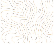
The next image to the right shows the image file after the elevations have been assigned. Note that the contour lines alternate in color indicating that the assignments are correct. This alternating color method works better than turning on the elevation values themselves. This should be used as a check. The problem is that the default zero values are overwritten without being refreshed so that they can quickly become crowded and illegible.

Inspect your work again carefully. If you have made an error in the elevation assignment, it is no problem to go back and correct the error. When you are satisfied that your file is error free, save the vector file by choosing "File | Save Vector As" and selecting "Arc View Shape File".

Once this is complete, you can open the file using BLACKART. BLACKART will automatically perform the contour line interpolation according to the parameters that you set in the program. This is pretty easy to do. In BLACKART, select File | Open. Select the "shape" option and open your .shp file produced by WinTopo. (Note: WinTopo will actually produce three files. In addition to the .shp file, there will be a .shx and a .dbf files. BLACKART needs data from all three files in order to build the input array. It does not matter what directory these files are in, as long as they are all in the same directory.)

When you open the file, you will be presented with a dialog box. Enter the number of iterations that you want to run. There are two choices: LSQR iterations and Laplacian iterations. The Laplacian iterations is the number of passes that the central difference approximation solver will make to compute an initial solution of the problem. This initial solution will be a low quality DEM that can be computed cheaply. This initial solution is used by the LSQR solver to produce the high quality DEM. The central difference solver is fast, so it is best to use a lot of iterations. 10,000 is not too many for most files.

The second entry controls the number of iterations used by the slower but better LSQR solver. Again, it is not possible to specify too many iterations. However, the larger the number, the longer the program will take to compute. Thousands of iterations are usually required to produce a good result but this will depend on the size of your input file and the characteristics of the topography being interpolated. When you have entered the data, submit it. Now select "Run | Run BLACKART". You will see progress bars and information in the dialog box about your run.

When the program computes successfully, you can view a 2D rendering of your DEM by selecting "View | View Image". If you are happy with the result, you can output your file as a USGS ASCII DEM or in ASCII xyz format. If you choose "File | Save ASCII DEM" you will be presented with another dialog box after entering the file name. You will be prompted for georeferencing information for your DEM. After you have entered this data, select "Submit" and save your DEM. You should now be able to import the DEM into any GIS application such as 3DEM, MicroDEM, Global Mapper, etc. The instructions for using the program are listed in the help file.

The final image shown is a 152 by 188 elevation posting DEM prepared from the input file shown above using BLACKART. Note the complete absence of terracing, hilltop plateaus, pits, and other unwanted features common to other less capable interpolation algorithms. (If you do not understand the importance of this, compare this image with the one produced by R2V in my previous article.)

With the simple tools outlined in this article, and a lot of patient work you should be able to produce DEMs for any part of the world for which digital or paper topographical maps are available. With the advent of global SRTM coverage, this may be less important in the future than it has been in the past. At 90m resolution however, SRTM leaves a lot to be desired for many applications. Contour line interpolation methods for producing DEMs should still have a place for some time to come.